How to Lock or Unlock Cells in Excel: A Beginner’s Guide

Do you need to protect certain cells in your Excel worksheet? Or maybe you want to lock all the cells except for a few that you can still edit. In any case, locking cells in Excel is easy to do, but you need to know the right steps. This article has tons of screenshots, plus step-by-step instructions and output to illustrate each point. Read on for a beginner’s guide to lock cells in Excel.
How to Prevent a Range of Cells in Excel from Being Updated
One of the most common tasks that you will do when you’re working with data in Excel is to lock certain cells. This can be helpful if you want to protect certain information from being edited or deleted. Here’s how to do it:
Step 1. First, open up the Excel worksheet that you want to work with.
Step 2. If your worksheet is already protected from editing, you’ll need to unprotect it first so that it can be freely modified.
To unprotect your worksheet in Excel, simply go to the “Review” tab and select “Unprotect Sheet”. It may request you to supply the password.

Step 3. Click the triangle icon in the upper left corner to select all of your sheet’s cells.
Step 3 through 5 is intended to ensure that none of the cells are locked once you’ve protected the workbook. This is necessary for determining which cells should be locked later.

Step 4. Click the popup launcher of “Alignment” or “Font” under the “Home” tab.

This will bring up the “Format Cells” window that includes a tab called “Protection”. Click it.

Step 5. Uncheck the box next to “Locked”, and then click “OK” to save your changes.

Step 6. Now it’s time to pick the cells you wish to lockdown once protection is enabled.
If you want to lock down an entire column or row then just click on that section of the spreadsheet. If you want to select a certain range, you can do this by clicking and dragging your cursor over the cells, or by using the keyboard shortcuts Ctrl+Click for individual cells or Shift+Click to select a range of cells.
In this example, we will lock cells A1 through B2.
Step 7. Once the cells are selected, click the popup launcher of “Alignment” (or “Font”) once again to display the window.
The previous step, we unchecked it to make the whole worksheet unlock. We must now change the status from uncheck to check by checking the box labeled “Locked”, to make A1 through B2 lock.

Step 8. Click on the “Review” tab and then select the “Protect Sheet” command from the menu. Enter a password if you want to password protect the cells. After that, click “OK”.
We recommend that you should create a password, as others only need to click the “Unprotect Sheet” button to edit it normally if you don’t.

Step 9. Save the workbook. If your operations are identical to the ones above, you will not be able to modify any cell from A1 to B2, and cells outside of this range can now be changed at leisure.
How to Ensure That Only a Few Cells Remain Editable
When your intention was to lock all but a few, here’s how to do.
Step 1. Open your Excel workbook and click on the sheet you want to lock.
Step 2. If the sheet is protected from editing, you’ll need to click on “Unprotect Sheet” on the “Review” tab to unprotect it first.

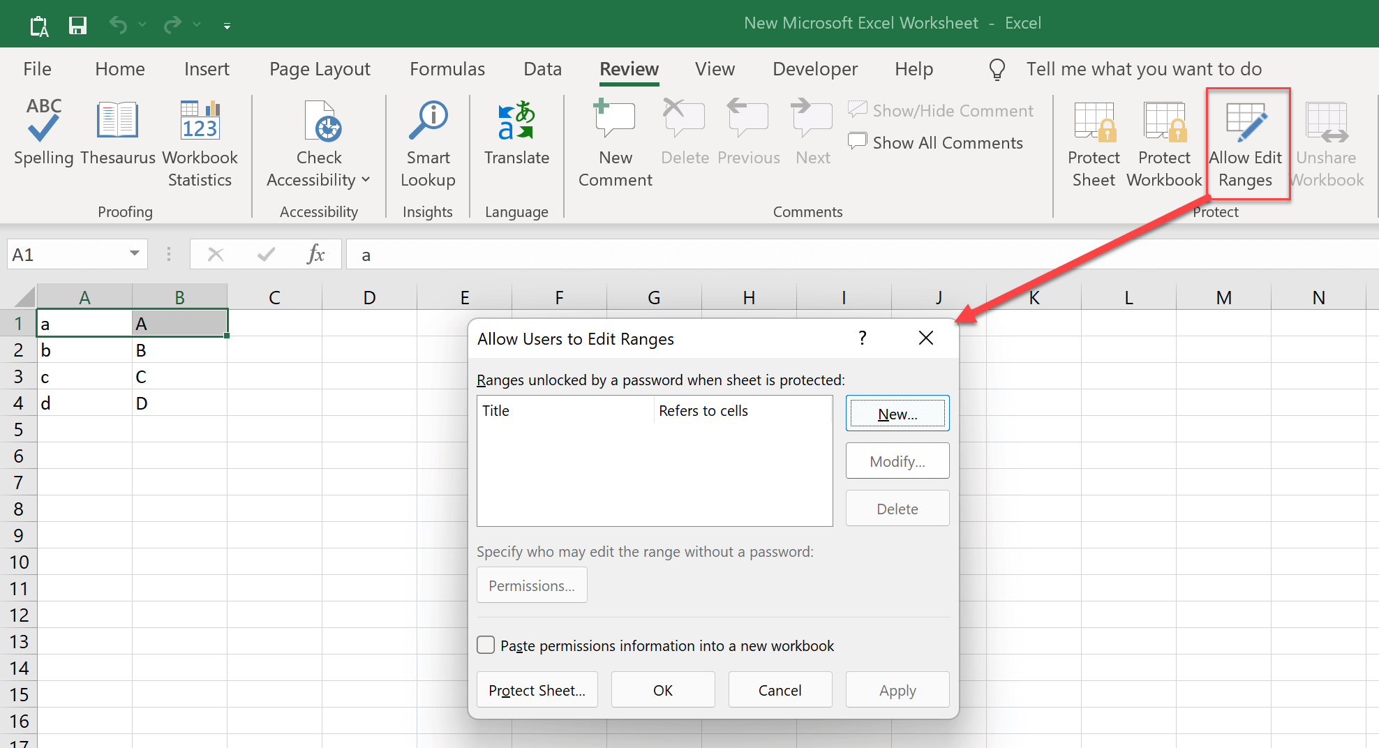
Step 3. With your mouse, select the cells that you want to allow edit, and then click on “Allow edit ranges” in order for the “Allow Users to Edit Ranges” window to appear.
In this example, cells A1 through B1 will be selected.

Step 4. Click on the “New” button to add a range. Under the “Title” section, you can give this range a name that you can easily understand. Under the “Refers to cells” section you’ll see that it’s shown the cells you chose.
You can also create a range password that allows only editing after entering it. The range password differs from the unprotecting password. Others with a “range password” but no “unprotection password” may only modify the cells you allow, and they may not unprotect the whole worksheet unless you use the same two passwords.

Step 5. Click on “OK” to save the changes and close the “New Range” window, and then click on “OK” again to close the “Allow Users to Edit Ranges” window.
Step 6. Go to the “Review” tab, then select the “Protect Sheet” button on your spreadsheet’s toolbar to lock the sheet.

Step 7. Save the Excel document. You’ll see that the lock is placed on all cells exexcept for A1 to B1, which means that A1 and B1 are allowed editing, but all other cells are locked for changes.
Now that you know how to lock or unlock cells in Excel, you can better protect your data from accidental changes or deletions.
If I Forgot the Editing Password, How Do I Unprotect My Sheet?
Passwords do increase security, but they can be inconvenient if you forget them. Fortunately, removing the edit protection password is a lot easier than hacking through open protection!
If for any reason, though, you lock yourself out by forgetting your editing password, the most straightforward solution is to copy the data to a new worksheet.
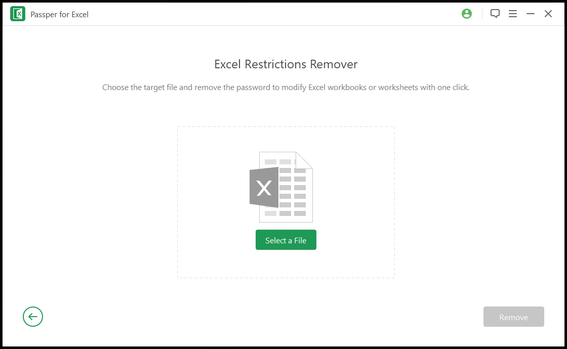
Alternatively, there are Excel Restrictions Removers, such as Passper for Excel, to assist you in removing restrictions with a single click. The time it takes to remove spreadsheet editing limitations has nothing to do with the password’s complexity. Regardless of how complicated the password is, the program can remove all workbook restrictions in 1 second.
Editor’s words
Locking cells in Excel is a useful tool that can be used to keep values from unexpected changes, but it’s not always clear how to do this. We hope these steps will help you lock down the values of any cell on your spreadsheet and make sure they stay there until you (or an authorized person) change them yourself. If anything about locking cells seems unclear or if you have other questions, feel free to leave us comments below.


